Documentation Index
Fetch the complete documentation index at: https://pycrm.xyz/llms.txt
Use this file to discover all available pages before exploring further.
Q-Learning in Letter World
This guide demonstrates how to train an agent using Q-learning with RM/CRMs in the Letter World environment.
Environment Overview
The Letter World environment consists of a 3×7 grid where:
- The agent starts at position (1,3)
- Letter ‘A’ appears at position (1,1)
- Letter ‘C’ appears at position (1,5)
- When the agent visits ‘A’, it may randomly change to ‘B’ with 50% probability
- The goal is to first visit ‘A’ (incrementing a counter), then visit ‘C’ to receive a positive reward
Setting Up the Environment
First, let’s create the environment components:
from examples.introduction.core.ground import LetterWorld
from examples.introduction.core.label import LetterWorldLabellingFunction
from examples.introduction.core.machine import LetterWorldCountingRewardMachine
from examples.introduction.core.crossproduct import LetterWorldCrossProduct

# Initialize environment components
ground_env = LetterWorld()  # Base grid world environment
lf = LetterWorldLabellingFunction()  # Labels events like seeing symbols A, B, C
crm = LetterWorldCountingRewardMachine()  # Defines rewards based on symbol sequence
cross_product = LetterWorldCrossProduct(
    ground_env=ground_env,
    crm=crm,
    lf=lf,
    max_steps=500,  # Maximum steps per episode before termination
)
Q-Learning Implementation
The Q-learning algorithm maintains a table of state-action values and updates them based on the rewards received:
import time
from collections import defaultdict
import numpy as np
from tqdm import tqdm
import matplotlib.pyplot as plt

# Initialize the Q-table as a defaultdict to store state-action values
q_table = defaultdict(
    lambda: np.zeros(cross_product.action_space.n)
)

# Q-learning hyperparameters
EPISODES = 5000       # Total training episodes
LEARNING_RATE = 0.1   # Alpha: how quickly we update Q-values with new information
DISCOUNT_FACTOR = 0.99  # Gamma: importance of future rewards vs immediate rewards
EPSILON = 0.1         # Exploration rate: probability of taking random action

# Track total rewards for visualization
all_returns = []

# Train the agent over multiple episodes with progress bar
pbar = tqdm(range(EPISODES))
for episode in pbar:
    obs, _ = cross_product.reset()
    episode_return = 0
    done = False

    # Run a single episode
    while not done:
        # Epsilon-greedy action selection
        if np.random.random() < EPSILON or np.all(q_table[tuple(obs)] == 0):
            action = np.random.randint(cross_product.action_space.n)
        else:
            action = int(np.argmax(q_table[tuple(obs)]))

        # Take action and observe result
        next_obs, reward, terminated, truncated, _ = cross_product.step(action)
        episode_return += reward
        done = terminated or truncated

        # Q-learning update
        # Q(s,a) = Q(s,a) + α * [r + γ * max_a' Q(s',a') - Q(s,a)]
        if done:
            td_target = reward  # No future rewards if episode is done
        else:
            td_target = reward + DISCOUNT_FACTOR * np.max(q_table[tuple(next_obs)])

        td_error = td_target - q_table[tuple(obs)][action]
        q_table[tuple(obs)][action] += LEARNING_RATE * td_error

        # Move to next state
        obs = next_obs

    # Record episode return
    all_returns.append(episode_return)

    # Update progress bar with recent average return
    if episode % 10 == 0:
        pbar.set_description(
            f"Episode {episode} | Ave Return: {np.mean(all_returns[-10:]):.2f}"
        )
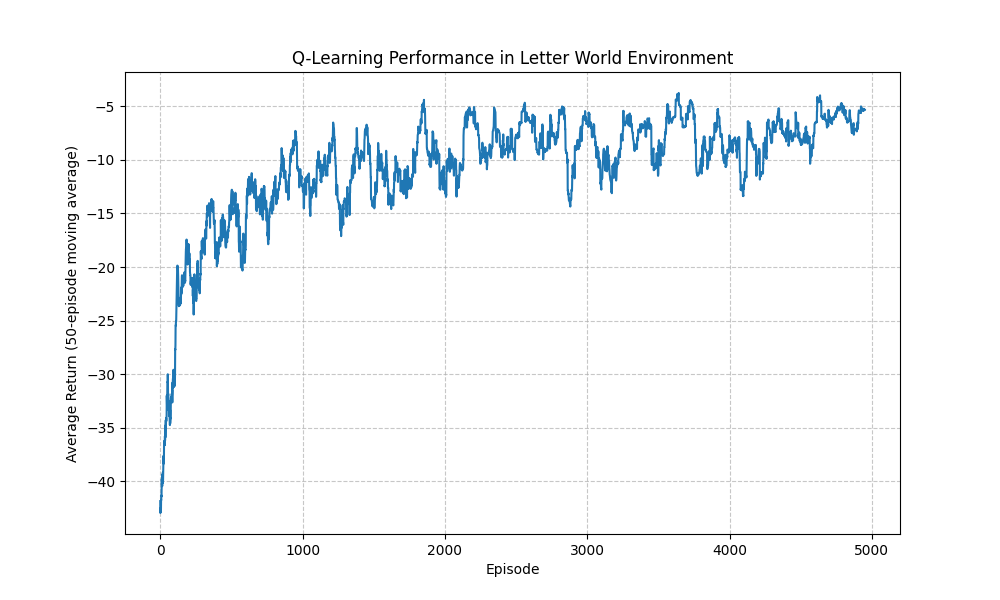
Training Progress Visualization
After training, we can visualize the agent’s learning progress:
# Visualize training progress
plt.figure(figsize=(10, 6))
all_returns = np.array(all_returns)

# Apply moving average for smoothing (window size = 50)
smoothed_returns = np.convolve(all_returns, np.ones((50,)) / 50, mode="valid")

plt.plot(smoothed_returns)
plt.title('Q-Learning Performance in Letter World Environment')
plt.xlabel('Episode')
plt.ylabel('Average Return (50-episode moving average)')
plt.grid(True, linestyle='--', alpha=0.7)
plt.savefig('q-learning.png')  # Save figure before showing
plt.show()
Demonstrating the Learned Policy
After training, we can observe how the agent behaves with its learned policy:
# Demonstrate learned policy
print("\nDemonstrating learned policy...")

for ep in range(3):  # We'll just show 3 episodes as example
    print(f"\nEpisode {ep+1}")
    obs, _ = cross_product.reset()
    done = False
    total_reward = 0
    step_count = 0

    # Render initial state
    cross_product.render()

    while not done:
        # Display current state and Q-values
        print(f"State: {obs}, Q-values: {q_table[tuple(obs)]}")

        # Select action (mostly greedy with small exploration)
        if np.random.random() < 0.1 or np.all(q_table[tuple(obs)] == 0):
            action = np.random.randint(cross_product.action_space.n)
            print(f"Taking random action: {action}")
        else:
            action = int(np.argmax(q_table[tuple(obs)]))
            print(f"Taking greedy action: {action}")

        # Execute action
        next_obs, reward, terminated, truncated, _ = cross_product.step(action)
        total_reward += reward
        step_count += 1

        print(f"Reward: {reward}, Cumulative: {total_reward}")

        done = terminated or truncated
        obs = next_obs

        # Render environment after action
        cross_product.render()

        # Brief pause for visualization
        time.sleep(0.5)

    print(f"Final state: {obs}")
    print(f"Episode {ep+1} complete. Total reward: {total_reward}, Steps: {step_count}")
Sample Output
When running the demonstration, you’ll see output similar to this:
Demonstrating learned policy...

Episode 1
+-------------+
|. . . . . . .|
|A . x . . C .|
|. . . . . . .|
+-------------+
State: [0 1 3 0 0], Q-values: [-0.15461255 -0.1        -0.11046881 -0.1       ]
Taking greedy action: 0
Reward: -0.1, Cumulative: -0.1
+-------------+
|. . . . . . .|
|A . . x . C .|
|. . . . . . .|
+-------------+
State: [0 1 4 0 0], Q-values: [-0.1        -0.1        -0.1         0.03374291]
Taking greedy action: 3
Reward: -0.1, Cumulative: -0.2
+-------------+
|. . . . . . .|
|A . . . x C .|
|. . . . . . .|
+-------------+
State: [0 1 5 0 0], Q-values: [-0.1        -0.1        -0.1        -0.1       ]
Taking greedy action: 0
Reward: -0.1, Cumulative: -0.3
+-------------+
|. . . . . . .|
|A . . . . x .|
|. . . . . . .|
+-------------+
State: [0 1 6 0 0], Q-values: [ 0.03603047 -0.1        -0.1        -0.1       ]
Taking greedy action: 0
Reward: -1.0, Cumulative: -1.3
Final state: [0 1 6 0 0]
Episode 1 complete. Total reward: -1.3, Steps: 4
Understanding the Algorithm
The Q-learning algorithm:
- Explores vs. Exploits: Uses an epsilon-greedy strategy to balance exploration (random actions) and exploitation (best known actions)
- Updates Q-values: After each action, updates the Q-value based on the reward received and the maximum future Q-value
- Learning Rate: Controls how quickly the agent updates its Q-values with new information
- Discount Factor: Determines the importance of future rewards compared to immediate rewards
In the Letter World environment, the agent needs to learn that:
- Visiting position ‘A’ is necessary to increment a counter
- After visiting ‘A’, the agent must navigate to position ‘C’ to receive a positive reward
- Navigation should be efficient to minimize negative step penalties
The learning curve shows that:
- Initial performance is poor as the agent explores randomly
- Performance improves rapidly as it discovers the optimal sequence
- Fluctuations occur as the agent balances exploration and exploitation
- Eventually, the agent converges toward an optimal policy
Conclusion
This example demonstrates how Q-learning can be used with RM/CRMs to train an agent to follow specific sequential tasks. The Letter World environment illustrates how CRMs can effectively model tasks that require remembering past events.
For more complex environments, you might need to adjust hyperparameters or use more sophisticated reinforcement learning algorithms, but the same CRM framework can be applied.
Next Steps